Index & Match Formula in Excel

Index & Match are very powerful lookup formula in Excel. Many of you will be familiar with the vlookup formula but Index & Match beats vlookup in many aspects and that’s the reason it’s one of the favorite for Data Analytics Professionals working on Excel or Google Spreadsheet.

Index:

This is a simple formula which takes input as array range and the row, column value and returns the corresponding value, Here is an example dataset: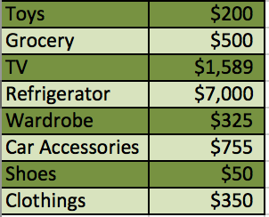

Apply Index on this dataset for cell value (3,2)

=INDEX(A2:B9,3,2)

A2:B9 - Array Range of the dataset

3 - Row value

2-Column value

Return Value:

$1589

Match:

This formula returns the numeric value based on the position of lookup value within the specified range defined by user. Let’s understand this

In the above dataset let’s apply Match Function and find the position of “Wardrobe” item in the list

=MATCH(A6,A2:A9,0)

A6 - is the “Wardrobe” Cell Value

A2:A9 - Array range under which the value has to be searched

0 - Match Type

Return Value:

5

So this is the value where Wardrobe item is located

Index & Match used in Conjunction:

Let’s find the value of Refrigerator using index & match formula:

=MATCH(A5,A2:A9,0)

This formula will return the row position of item Refrigerator i.e. 4

Now incorporate this formula within the Index

=INDEX(A2:B9,MATCH(A5,A2:A9,0),2)

So, A2:B9 - Array Range for dataset

MATCH(A5,A2:A9,0) - Will return value of 4, which is row number

2 - is the column whose value is desired

The return value of the Index function above is $7000, which is the amount of the item Refrigerator.