Dynamic Dashboards in Excel
Dashboards are really a great tool to Visualize the data and help to find insights from the datasets. it helps to organize and present the data in a easy graphical format. There are lot of tools available in market which help you to visualize your dataset in a pretty decent formats. However Excel & Google Spreadsheets are the most widely tool for data analytics across the industries.
In my this post I’m going to show you how to build an Interactive and User Friendly Dashboard for your Yearly Expenditure without much of effort using Excel or Google Spreadsheet.
Here is the Data used for building the dashboard, Open a new Google Spreadsheet and paste this data in the first two rows.

Firstly, You need to think how your dashboard should look like and what are User Interactions fields would be required, So in this case we would just need to filter by “Year” and view our Yearly Expenditure.
Let’s have a Cell with drop-down values for Years i.e. 2015 & 2016.
Select Cell A6 and Go to Data > Data Validation and Under field “Criteria” select the range of Year column where data is pasted above, i.e. A2:A3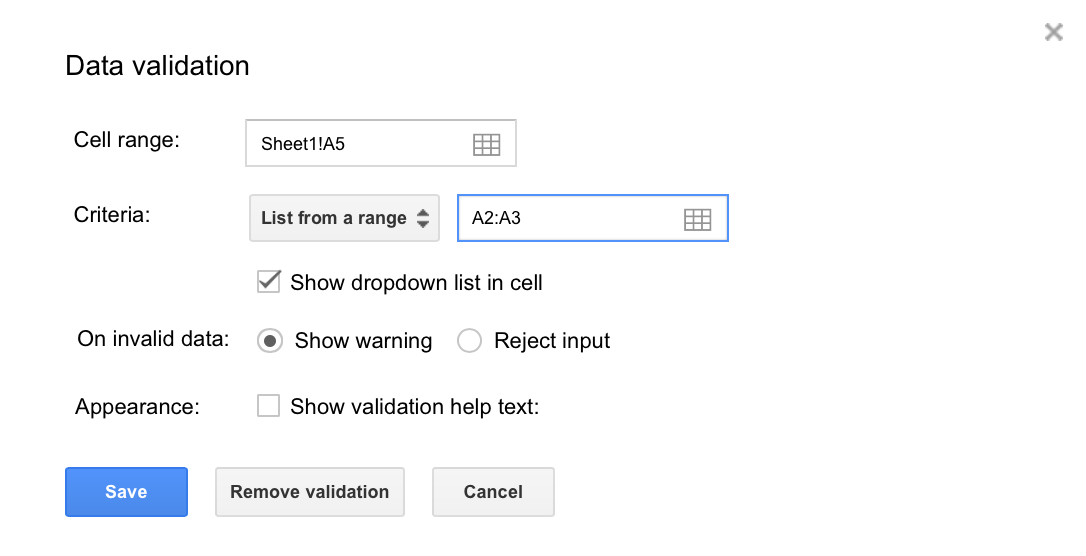
Will need to pull the corresponding values for all the expenses from the above two rows as per the year selected in Cell A6.
Read this post for Index & Match function before you go further
This is the Formula to be used for each of the cell to get the expenses as per the selected year:
=INDEX($B$2:$N$3,MATCH($A$6,$A$2:$A$3,0),column())

Let’s dissect the above formula:
MATCH($A$6,$A$2:$A$3,0)
This formula will look for the “Year” selected in cell A6 and will match with the data rows above and returns the row number, For example: if Year selected is 2015 then return value is 1 and if it’s 2016 then return value is 2
=INDEX($A$2:$N$3,MATCH($A$6,$A$2:$A$3,0),column())
Index will return the value of the cell and row specified, so for example the cell value is returned based upon the above formula Match return value 1 or 2 and the last parameter column(). For example: Grocery(B6) value if Year selected is 2015 then Match formula returns 1 and the column() value is 2, so Index will return the cell value of (1,2) i.e. 2500
Now Change the Year from dropdown in A6 and see how the corresponding cell values changes in row#6


Build the Dashboard as per the Chart of your Choice, In this Dashboard I will have Bar, Area, Table & Pie Chart to visualize my data.
Select the Data Range for Row#6 only one single row and create the Dashboard. For example for a Bar chart, select the data range as follows:
B5:N6

For all other graphs also select the same Data range i.e. B5:N6 and now change the Year value from cell A6 and see how the dashboard changes dynamically.